Classification in the wild

I have been working on ML-based projects for the last 5+ years. During my career, I worked on different projects, startups, big companies, won a few competitions, and wrote a few papers. I have also launched the Catalyst – a high-level framework on top of PyTorch to boost my productivity as a deep learning practitioner. With such a path, I have recently decided to write a series of posts about deep learning “general things”. After a few ideas, I have decided to start from ML evaluation techniques and metrics: how to understand them? when to use them? In such a case, today, I would like to dive into classification metrics in deep learning and discuss a few tricks, which could boost your classification pipeline performance.

You can find all the examples below under this colab notebook.

Exp 01: typical classification

The classification task looks well-known for any deep learning practitioner. Long story short, we have some labeled data in (some-data, label) format and want to create a model, which could transfer some-extra-data to label for us. As an example, let’s review simple CIFAR10 classification:

import os
import torch
from torch import nn, optim
from torch.utils.data import DataLoader
from catalyst import dl, utils
from catalyst.contrib.datasets import CIFAR10
from catalyst.contrib.nn import ResidualBlock
from catalyst.data import transforms


# common
def conv_block(in_channels, out_channels, pool=False):
    layers = [
        nn.Conv2d(in_channels, out_channels, kernel_size=3, padding=1),
        nn.BatchNorm2d(out_channels),
        nn.ReLU(inplace=True),
    ]
    if pool:
        layers.append(nn.MaxPool2d(2))
    return nn.Sequential(*layers)


def resnet9(in_channels: int, num_classes: int, size: int = 16):
    sz, sz2, sz4, sz8 = size, size * 2, size * 4, size * 8
    return nn.Sequential(
        conv_block(in_channels, sz),
        conv_block(sz, sz2, pool=True),
        ResidualBlock(
            nn.Sequential(conv_block(sz2, sz2), conv_block(sz2, sz2))
        ),
        conv_block(sz2, sz4, pool=True),
        conv_block(sz4, sz8, pool=True),
        ResidualBlock(
            nn.Sequential(conv_block(sz8, sz8), conv_block(sz8, sz8))
        ),
        nn.Sequential(
            nn.MaxPool2d(4),
            nn.Flatten(),
            nn.Dropout(0.2),
            nn.Linear(sz8, num_classes),
        ),
    )


# data
utils.set_global_seed(42)
transform = transforms.Compose(
    [
        transforms.ToTensor(),
        transforms.Normalize((0.485, 0.456, 0.406), (0.229, 0.224, 0.225)),
    ]
)
train_data = CIFAR10(
    os.getcwd(), train=True, download=True, transform=transform
)
valid_data = CIFAR10(
    os.getcwd(), train=False, download=True, transform=transform
)

# loaders
loaders = {
    "train": DataLoader(train_data, batch_size=32, num_workers=0),
    "valid": DataLoader(valid_data, batch_size=32, num_workers=0),
}

# model, criterion, optimizer, scheduler
model = resnet9(in_channels=3, num_classes=10)
criterion = nn.CrossEntropyLoss()
optimizer = optim.Adam(model.parameters(), lr=1e-3)
scheduler = optim.lr_scheduler.MultiStepLR(optimizer, [5, 8], gamma=0.3)

# model training
runner = dl.SupervisedRunner(
    input_key="features",
    output_key="logits",
    target_key="targets",
    loss_key="loss",
)
runner.train(
    model=model,
    criterion=criterion,
    optimizer=optimizer,
    scheduler=scheduler,
    loaders=loaders,
    logdir="./logs/exp01",
    num_epochs=10,
    valid_loader="valid",
    valid_metric="accuracy01",
    minimize_valid_metric=False,
    verbose=True,
    callbacks=[
        dl.AccuracyCallback(
            input_key="logits", target_key="targets", num_classes=10
        ),
    ],
    load_best_on_end=True,
)

To sum up an example above:

• we create resnet9 network
• train it on CIFAR10 for 10 epochs
• with CE loss, Adam optimizer, MultiStep scheduler
• and accuracy as a validation metric

This example looks like a very common classification pipeline.
Could we do it better? Let’s check it out!

Exp 02: focal loss

Starting from a simple improvement, let’s introduce FocalLoss instead of CE. For a long review, please read the original paper, for a short review: thanks to per-sample loss reweighing based on the difference between true and predicted probabilities, FocalLoss better handles class imbalance, focusing on poorly distinguishable classes. As a result, it gives better performance for classification tasks with heavy class imbalance (real-world case, not CIFAR one). What is more important, it doesn’t introduce any additional complexity into your pipeline. So let’s check it out:

import os
import torch
from torch import nn, optim
from torch.utils.data import DataLoader
from catalyst import dl, utils
from catalyst.contrib.datasets import CIFAR10
from catalyst.contrib.nn import FocalLossMultiClass, ResidualBlock
from catalyst.data import transforms


# common
def conv_block(in_channels, out_channels, pool=False):
    layers = [
        nn.Conv2d(in_channels, out_channels, kernel_size=3, padding=1),
        nn.BatchNorm2d(out_channels),
        nn.ReLU(inplace=True),
    ]
    if pool:
        layers.append(nn.MaxPool2d(2))
    return nn.Sequential(*layers)


def resnet9(in_channels: int, num_classes: int, size: int = 16):
    sz, sz2, sz4, sz8 = size, size * 2, size * 4, size * 8
    return nn.Sequential(
        conv_block(in_channels, sz),
        conv_block(sz, sz2, pool=True),
        ResidualBlock(
            nn.Sequential(conv_block(sz2, sz2), conv_block(sz2, sz2))
        ),
        conv_block(sz2, sz4, pool=True),
        conv_block(sz4, sz8, pool=True),
        ResidualBlock(
            nn.Sequential(conv_block(sz8, sz8), conv_block(sz8, sz8))
        ),
        nn.Sequential(
            nn.MaxPool2d(4),
            nn.Flatten(),
            nn.Dropout(0.2),
            nn.Linear(sz8, num_classes),
        ),
    )


# data
utils.set_global_seed(42)
transform = transforms.Compose(
    [
        transforms.ToTensor(),
        transforms.Normalize((0.485, 0.456, 0.406), (0.229, 0.224, 0.225)),
    ]
)
train_data = CIFAR10(
    os.getcwd(), train=True, download=True, transform=transform
)
valid_data = CIFAR10(
    os.getcwd(), train=False, download=True, transform=transform
)

# loaders
loaders = {
    "train": DataLoader(train_data, batch_size=32, num_workers=0),
    "valid": DataLoader(valid_data, batch_size=32, num_workers=0),
}

# model, criterion, optimizer, scheduler
model = resnet9(in_channels=3, num_classes=10)
criterion = FocalLossMultiClass()
optimizer = optim.Adam(model.parameters(), lr=1e-3)
scheduler = optim.lr_scheduler.MultiStepLR(optimizer, [5, 8], gamma=0.3)

# model training
runner = dl.SupervisedRunner(
    input_key="features",
    output_key="logits",
    target_key="targets",
    loss_key="loss",
)
runner.train(
    model=model,
    criterion=criterion,
    optimizer=optimizer,
    scheduler=scheduler,
    loaders=loaders,
    logdir="./logs/exp02",
    num_epochs=10,
    valid_loader="valid",
    valid_metric="accuracy01",
    minimize_valid_metric=False,
    verbose=True,
    callbacks=[
        dl.AccuracyCallback(
            input_key="logits", target_key="targets", num_classes=10
        ),
    ],
    load_best_on_end=True,
)

While we haven’t significantly improved CIFAR10 results, FocalLoss usually helps with more practical cases. Finally, a short trick, I also want to mention - multi-criterion usage:

criterion = {
    "ce": nn.CrossEntropyLoss(),
    "focal": FocalLossMultiClass()
}

callbacks = [
    dl.CriterionCallback(
        input_key="logits",
        target_key="targets",
        metric_key="loss_ce",
        criterion_key="ce",
    ),
    dl.CriterionCallback(
        input_key="logits",
        target_key="targets",
        metric_key="loss_focal",
        criterion_key="focal",
    ),
    dl.MetricAggregationCallback(
        metric_key="loss",
        metrics={"loss_ce": 0.5, "loss_focal": 0.5},
        mode="weighted_sum",
    ),
    dl.OptimizerCallback(metric_key="loss"),
]

This approach gives you a way to balance straightforward classification (with CE loss) and imbalance-focused one (with FocalLoss).

Exp 03: classification metrics

Okay, as we have seen, we could “improve” our accuracy performance a bit thanks to FocalLoss. But there are a few additional classification metrics to understand your model better:

• precision - shows model assurance in label prediction. For example, suppose precision is high, and the model predicts some label L for some input I. In that case, there is a high probability that I is actually L.
• recall - shows model ability to find all class instances in the data stream. Of course, the high recall does not mean that all model predictions will be accurate enough, but it gives us a high probability of covering all class instances.
• f-score - is a harmonic mean between precision and recall. Hence, it could be seen as a unified score to understand the model’s ability to find all relevant classes in the data stream (recall) and label them correctly (precision). Moreover, f-score beta parameter allows us to preference for precision or recall during aggregation.

Additionally, there are two more things, which are essential to check during model training and predictions:

• support - just a simple number of samples per class. It seems oblivious, but the more data points you have - the confident insight you can find. And sometimes, even if you have a large dataset with a wide variety of classes, there could be classes with only a few examples, leading to unpredictable results during training and evaluation. Adding a support metric to your pipeline gives you a simple way to “validate” the dataset during training.
• confusion matrix - easy to follow resume of your classification model ability to distinguish different classes. While it, obliviously, helps you analyze model correctness (confusion matrix diagonal), it also gives you important insight into classes distribution and labeling. There were several cases in my practice when confusion matrix helped to find incorrect labeling during dataset update - just reviewing the classes interactions anomalies on confusion matrix.

Let’s add them to our pipeline:

import os
import torch
from torch import nn, optim
from torch.utils.data import DataLoader
from catalyst import dl, utils
from catalyst.contrib.datasets import CIFAR10
from catalyst.contrib.nn import ResidualBlock
from catalyst.data import transforms


# common
def conv_block(in_channels, out_channels, pool=False):
    layers = [
        nn.Conv2d(in_channels, out_channels, kernel_size=3, padding=1),
        nn.BatchNorm2d(out_channels),
        nn.ReLU(inplace=True),
    ]
    if pool:
        layers.append(nn.MaxPool2d(2))
    return nn.Sequential(*layers)


def resnet9(in_channels: int, num_classes: int, size: int = 16):
    sz, sz2, sz4, sz8 = size, size * 2, size * 4, size * 8
    return nn.Sequential(
        conv_block(in_channels, sz),
        conv_block(sz, sz2, pool=True),
        ResidualBlock(
            nn.Sequential(conv_block(sz2, sz2), conv_block(sz2, sz2))
        ),
        conv_block(sz2, sz4, pool=True),
        conv_block(sz4, sz8, pool=True),
        ResidualBlock(
            nn.Sequential(conv_block(sz8, sz8), conv_block(sz8, sz8))
        ),
        nn.Sequential(
            nn.MaxPool2d(4),
            nn.Flatten(),
            nn.Dropout(0.2),
            nn.Linear(sz8, num_classes),
        ),
    )


# data
utils.set_global_seed(42)
transform = transforms.Compose(
    [
        transforms.ToTensor(),
        transforms.Normalize((0.485, 0.456, 0.406), (0.229, 0.224, 0.225)),
    ]
)
train_data = CIFAR10(
    os.getcwd(), train=True, download=True, transform=transform
)
valid_data = CIFAR10(
    os.getcwd(), train=False, download=True, transform=transform
)

# loaders
loaders = {
    "train": DataLoader(train_data, batch_size=32, num_workers=0),
    "valid": DataLoader(valid_data, batch_size=32, num_workers=0),
}

# model, criterion, optimizer, scheduler
model = resnet9(in_channels=3, num_classes=10)
criterion = nn.CrossEntropyLoss()
optimizer = optim.Adam(model.parameters(), lr=1e-3)
scheduler = optim.lr_scheduler.MultiStepLR(optimizer, [5, 8], gamma=0.3)

# model training
runner = dl.SupervisedRunner(
    input_key="features",
    output_key="logits",
    target_key="targets",
    loss_key="loss",
)
runner.train(
    model=model,
    criterion=criterion,
    optimizer=optimizer,
    scheduler=scheduler,
    loaders=loaders,
    logdir="./logs/exp03",
    num_epochs=10,
    valid_loader="valid",
    valid_metric="f1/_micro",
    minimize_valid_metric=False,
    verbose=True,
    callbacks=[
        dl.AccuracyCallback(
            input_key="logits", target_key="targets", num_classes=10
        ),
        dl.PrecisionRecallF1SupportCallback(
            input_key="logits", target_key="targets", num_classes=10
        ),
        dl.ConfusionMatrixCallback(
            input_key="logits", target_key="targets", num_classes=10
        ),
    ],
    load_best_on_end=True,
)

There are a few crucial tricks to watch with these metrics. All of them could be computed both “per-class” or “aggregated” over the classes. “Per-class” results are crucial for model performance understanding cause there are many cases when your model could perform “well” in general and “worst than ever before” on the most important classes. For example, we could review some text classification model, which greatly works with greeting intents, but fails at toxic ones prediction, which could be much more valuable from a business perspective. “Aggregated” results are essential if you want to review model performance in only a few numbers quickly. There a three most common aggregation strategies:

• micro: all samples equally contribute to the final averaged metric,
• macro: all classes equally contribute to the final averaged metric,
• weighted: each classes' contribution is weighted by its size during averaging.

Another important note of the above metrics is that all their results are dataset-based, which means you couldn’t simply average the batch-based micro-metrics to get dataset-based micro statistics.

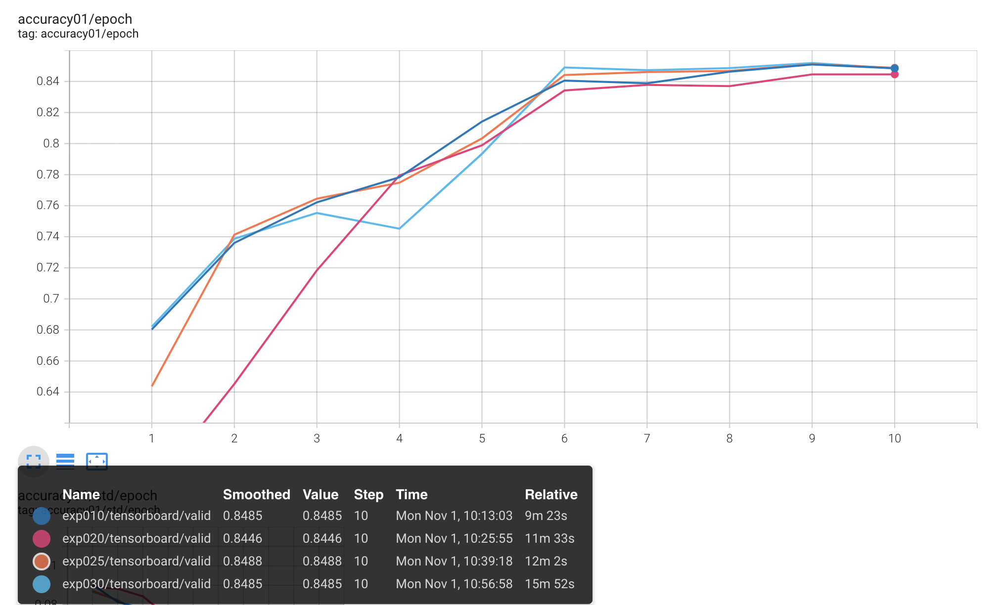
Tensorboard

As far as we have a large variety of different metrics, it’s much easier to use tensorboard to watch them all:

tensorboard --logdir ./logs

Inference & report

Additionally, there is also a way to represent all the above metrics in a user-friendly way to review the final model performance:

import numpy as np
from sklearn import metrics
from catalyst import utils

y_test = []
logits = []
loader = loaders["valid"]
for batch, prediction in zip(loader, runner.predict_loader(loader=loader)):
    _, y = batch
    y = y.detach().cpu().numpy()
    logits_ = prediction["logits"].detach().cpu().numpy()
    y_test.append(y)
    logits.append(logits_)

y_test = np.hstack(y_test)
logits = np.vstack(logits)
scores = torch.softmax(torch.tensor(logits), dim=1).detach().cpu().numpy()
y_pred = logits.argmax(axis=1)

df = utils.get_classification_report(y_true=y_test, y_pred=y_pred)
best_score_without_threshold = df["precision"]["accuracy"]
df

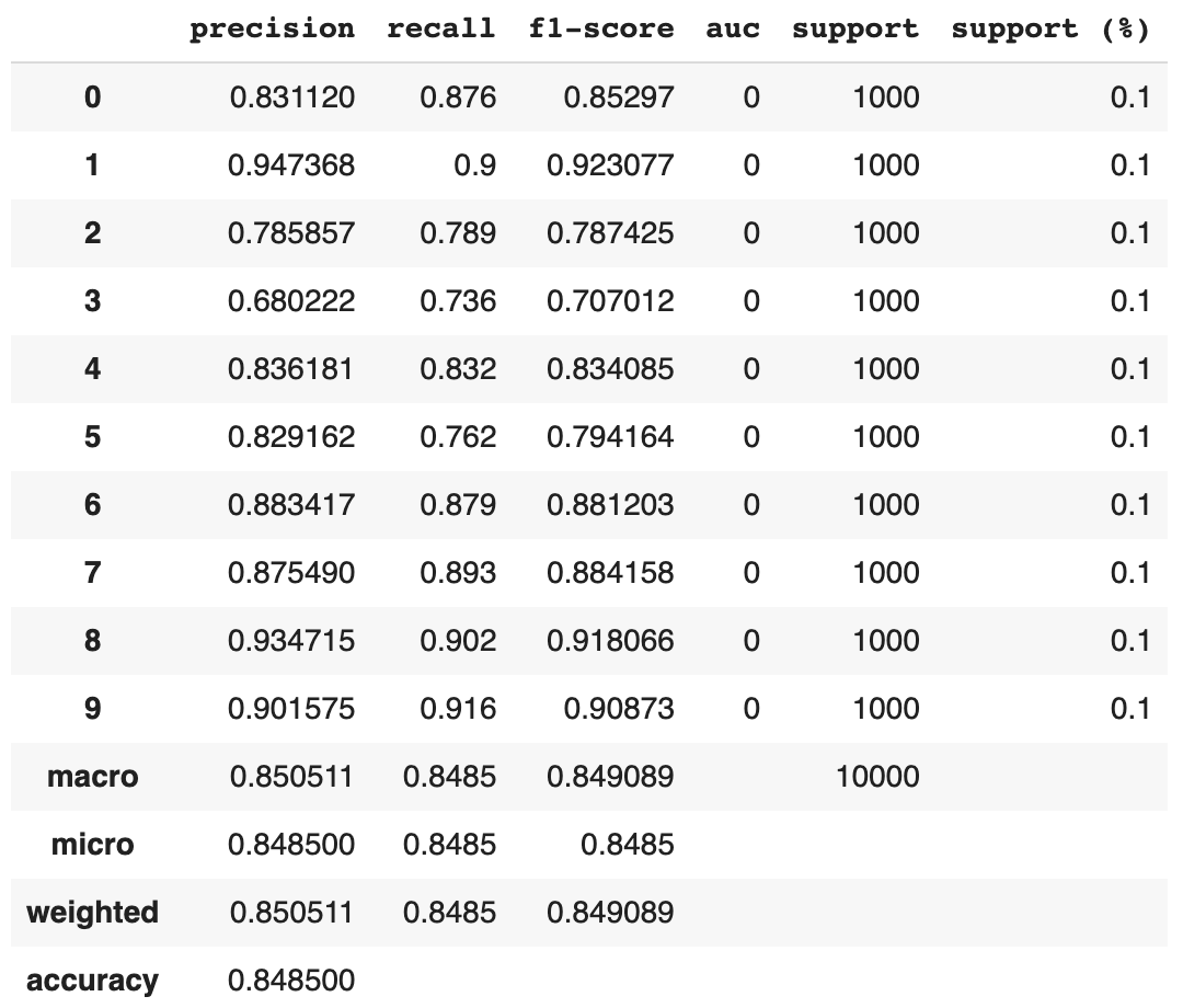
With such a classification report, it’s much easier to conclude the model’s final performance.

Thresholds

The last critical step I would like to mention in this tutorial is thresholds. While they are not fancy deep learning models, they give you a way to tune these models for your production cases without any additional learning. So, for example, you could set a threshold of 1.0 for some poor working class to stop the model from predicting it at all. As far as this is an essential practice in production deep learning, it is also included in the Catalyst:

(
    best_score_with_threshold,
    best_thresholds,
) = utils.get_best_multiclass_thresholds(
    scores=scores, labels=y_test, objective=metrics.accuracy_score
)

ratio = (
    best_score_with_threshold - best_score_without_threshold
) / best_score_without_threshold
print(
    f"Without Th: {best_score_without_threshold}\n"
    f"With Th: {best_score_with_threshold}\n"
    f"Improvement: {ratio}"
)

Without Th: 0.8485
With Th: 0.8516
Improvement: 0.003653506187389501

As you can see, we have been able to slightly improve our model performance even in such a simple setup as CIFAR (model learning on CIFAR is quite easy). Of course, there is a data leak during benchmarking because we were tuning and evaluating thresholds on the same test set, so in a real-world example, you have to split your dataset into train, valid, and test parts to prevent any data leaks. Nevertheless, even with such a strict evaluation setup, thresholds usage usually gives a critical 2–8% improvement for your metric on interest, which is huge.

Conclusion

So, to sum up, the main topics for this blog post:

• classification problem is still an open area for improvement (especially in the close vs. open sets domain, but this is another post),
• try the FocalLoss in your next experiment, if you have a class imbalance in your data (a pretty common case),
• use PrecisionRecallF1Support and ConfusionMatrix to analyze your model performance during training,
• use classification report to understand your final model classification performance,
• try thresholds during model deployment to tune the model for your special cases and improve the final performance.

If you want to dive deeper into this classification example, you could:

• use CIFAR100 instead of the default CIFAR10,
• check out one of our CV datasets available,
• try to adapt the same pipeline for NLP (Albert training example on TPUs),

or tune it for whatever classification problem you want ;)

Those were all the important steps in classification for this blog post. If you would like to check more deep learning best practices - subscribe for scitator & catalyst-team. Thanks for reading, and stay tuned for more!